Configuring joins by type
Siren Federate offers four join strategies: the hash join, the broadcast join, the index join, and the routing join.
By default, the Siren Federate query planner selects the most cost-effective join strategy based on the scenario, but you can also manually select the strategy that you prefer.
About join strategies
-
The hash join is a fully-distributed join strategy that is designed to join a large number of documents. It scales horizontally (based on the number of data nodes) and vertically (based on the number of CPU cores).
-
The broadcast join is the strategy to use when you are joining a large set of documents (the parent set) with a small to medium set of documents (the child set).
-
The index join is the strategy to use when you are joining a large set of documents (the parent set) with a small set of documents (the child set).
-
The routing join is the strategy to use when you want to join on the parent set’s
_idfield and there are more than one shard for the parent index distributed across more than one node in the cluster.
When to use a hash join
The hash join is best suited to scenarios where both parent and child sets are large or when the child set is large. A large set is, for example, a set of ten million tuples or more.
The hash join allows the processing of large amounts of data with minimal cost to the network performance.
Therefore, the hash join is useful in a cybersecurity use case, for example, where irregular machine events are being investigated.
|
A tuple is a single row composed of one or more columns, where one column is mapped to one field of a document. For example, a tuple could be a row composed of two elements such as the document identifier and the key value of the join condition. If a document has a multi-valued field, this will generate as many tuples as there are values. |
For more term definitions, see the Glossary.
When to use a broadcast join
The broadcast join is best suited to scenarios where the child set of documents (also known as the right-side set) is small or medium (up to a few millions).
Therefore, the broadcast join is useful in a commercial use case, for example, where the sales of a small number of selected products are being observed.
When to use an index join
The index join is best suited to scenarios where the child set of documents (also known as the right-side set) is small (up to a few thousands keys).
Therefore, the index join is useful in a social graph use case, for example, where you start with one person and try to expand his/her relations.
When to use a routing join
The routing join is best suited to scenarios where the join condition involves the parent set’s _id field; as it only works when using the default document routing strategy (the default _routing value is the document’s _id).
The routing join strategy partitions and shuffles the child set of documents based on the number of shards of the parent index. The performance of the routing join will increase with the number of shards in the parent index and with the number of data nodes in the cluster.
The performance of the routing join is optimal when the parent set of documents are located in one single concrete index. The performance of the routing join will decrease with the number of concrete indices as it will have to replicate the child set of documents to each parent index. In the worst case scenario, for example with a time series index, the routing join will behave like a broadcast join.
Also, the performance of routing join is better when the _id field contains only numeric values as it will simplify the encoding/decoding operations performed on that field.
Similarly to the broadcast join, the routing join can be useful in a commercial use case where the sales of a small number of products are being observed, and the sales reference the products using their _id. This permits some optimization of the routing join over the broadcast join (see the Partitioning data section).
Partitioning data
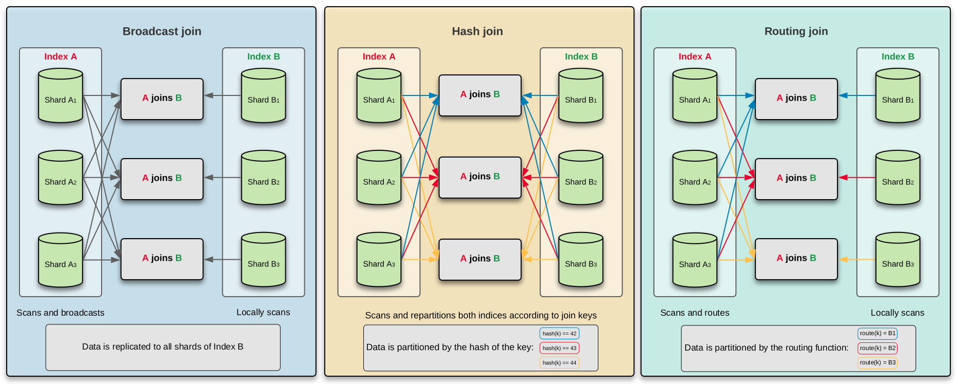
The difference between the broadcast join, the hash join, and the routing join lies in their approach to data partitioning.
In the following diagram, the broadcast join is shown sending data from the child set of documents (Index B) to every data node in the cluster. Therefore, each data node has the exact same input data as every other data node.
Data from the child set of documents (Index B) is sent only to data nodes that host shards of the parent set of documents (Index A). In addition, if data needs to be sent to two shards that are hosted on the same node, for example, a primary shard and a replica of Index A, then the data is sent only once to that node.
To further reduce data uploads, the routing join leverages Elasticsearch document routing. This allows to send data from the child set to only those nodes that host parent set’s shards that may contain a join match.
For this to happen, the join must be on the parent set’s _id field. By default, Elasticsearch uses the value of _id to determine on which shard a document is indexed. This permits to know a priori where a child set’s tuple must be uploaded for joining: if a parent set’s matching document exists, it can be only in the shards dictated by Elasticsearch’s document routing.
Finally, in a hash join, data from both sides is partitioned over the key and a data node receives only data with the same hash key.
To summarize, the hash join scales gracefully to process large amounts of data as the number of data nodes increases, thanks to the hash partitioning of the data.
In contrast, the broadcast and index join do not scale well because:
-
child data is duplicated across all of the nodes in the cluster, increasing network cost; and
-
a receiving node is subject to higher memory cost as the data increases.
The routing join lies somewhere in the middle in terms of scalability, but it is limited to join on the parent set’s _id field.
| Join strategy | Shuffle phase (data partitioning) | Build phase | Probe phase |
|---|---|---|---|
Broadcast join |
Copies of the input data (the child set of documents) are sent to every data node. |
A in-memory hash table is built over the input data. |
The |
Hash join |
Data from both sides is partitioned over the key and a data node receives only data with the same hash key. |
An in-memory hash table is built from one of the relations in the partition. |
The second relation is scanned and each value is probed against the hash table to find matches. |
Index join |
Copies of the input data (the child set of documents) are sent to every data node. |
An in-memory hash table is built over the input data. |
Each value is probed against the dictionary of the parent set to find matches. |
Routing join |
Data from the child set’s is partitioned over the key using a routing function, and a data node receives only its associated data. |
An in-memory hash table is built over the input data. |
The dictionary of |
Impact on performance
With a broadcast or an index join, uploading data to every data node in the cluster has an impact on the network load, the more data and nodes there are. In addition, the memory overhead on a node is linear with the size of the child set.
With the broadcast join, doc_values of the joined field of the parent set is scanned, while with the index join we perform a dictionary lookup. Indeed, with a small number of terms, the lookup is more efficient.
Compared to broadcast and index join, the routing join reduces the network overhead as the data of child set’s are partitioned and sent only to certain nodes. Since each node receives less data, the routing join also reduces the memory overhead compared to the broadcast join.
With a hash join, apart from the network load, the fact that the data is partitioned over the cluster also has an impact on the amount of memory needed. However, the created hash table is often smaller.
|
It is possible to change the parallelization of the hash join computation by using the
|
The Siren Query Planner performs a cost analysis to select the most suitable join strategy when none is specified by the user.
Example of the network, memory, and I/O cost of joins
A three-node cluster contains two indices with fields fieldA and fieldB, each field containing 15 million values. The field fieldA is a field from the parent set, and fieldB is a field from the child set.
In addition, each index has three primary shards and no replica. Consequently, one node has one shard of the index.
Hash and broadcast joins are two join strategies that scan the doc_values of joined fields. This scan is divided into the three categories that are most impacted:
-
Network: This exhibits the cost of transferring data between nodes;
-
I/O: This highlights the cost of reading data from the disk; and
-
Memory: This indicates the memory requirements when joining data.
Hash join
To join both indices over fields fieldA and fieldB with the hash join, the cost would be as follows:
-
I/O cost: The system scans
doc_valuesof each index before the shuffling phase. This represents a sequential scan of 15M + 15M = 30M values or 30M / 3 = 10M per node. -
Network cost: The system shuffles each index across the available data nodes. This represents a network transfer of 15M + 15M = 30M values across the cluster.
-
Memory cost: The system stores the projected data in (off-heap) memory from both child and parent sets. The total number of values stored in memory across the cluster is 15M + 15M = 30M, since there is no duplication when compared to the broadcast join. This represents 30M / 3 = 10M values per node.
Broadcast join
To join both indices over fields fieldA and fieldB with the broadcast join, the cost would be as follows:
-
I/O cost: The system scans
doc_valuesof each index and reads 15M + 15M = 30M values from both sides of the join. -
Network cost: The system shuffles the child index across data nodes hosting shards of the parent set. This represents a network transfer of 15M * 3 = 45M values across the cluster.
-
Memory cost: The system stores the projected data in (off-heap) memory. The number of values stored in off-heap memory is 15M on each node (values from
fieldB), which are also loaded into a hash table. This represents 30M on each node, thus a total of 90M values loaded into memory across the cluster.
Index join
To join both indices over fields fieldA and fieldB with the index join, the cost would be as follows:
-
I/O cost: The system scans
doc_valuesof the child set and reads 15M values. The system also performs 15M dictionary lookups on the parent index. -
Network cost: The system shuffles the child index across data nodes hosting shards of the parent set. This represents a network transfer of 15M * 3 = 45M values across the cluster.
-
Memory cost: The system stores the projected data in (off-heap) memory. The number of values stored in off-heap memory is 15M on each node (values from
fieldB), which are also loaded into a hash table. This represents 30M on each node, thus a total of 90M values loaded into memory across the cluster.
From this example, we can determine that the hash join strategy is less expensive on the system’s operations.
While the broadcast join outshines the hash join when the child index is small (since the parent index is not partitioned over the cluster), in the above case, the broadcast join does not scale very well because:
-
the child data is duplicated across all of the nodes in the cluster, increasing network cost; and
-
a receiving node is subject to higher memory cost as the data increases.
In contrast, the hash join scales gracefully to process large amounts of data as the number of data nodes increases, thanks to the hash partitioning of the data.
Routing join
The routing join can be used only if fieldA is _id. In that case, the cost would be as follows:
-
I/O cost: The system scans the parent set’s dictionary of
_ids and the child set’sdoc_valuesreading 15M + 15M = 30M values from both sides of the join. -
Network cost: The system shuffles the child index across data nodes hosting shards of the parent set, but a child’s value is uploaded on a data node only if this may lead to a join match. Assuming that the parent set’s shard are disjunct, each child’s value must be uploaded only once. This represents a network transfer of 15M values across the cluster.
-
Memory cost: The system stores the projected data in (off-heap) memory. Assume that the child’s value have been uniformly uploaded on the three nodes. Then the number of values stored in off-heap memory is 5M on each node (values from
fieldB), which are also loaded into a hash table. This represents 10M on each node, thus a total of 30M values loaded into memory across the cluster.
In this example, the routing join can compete with the hash join in terms of efficiency provided that we are joining on the parent set’s _id.
Requirements for executing a join
-
Ensure that the data type of the joined fields across index patterns is the same. For example, if you try to join a field from the pattern
index*, but the field is an integer inindex1while it is a keyword inindex2, an error will result. -
The following primitive data types are supported for joins based on a single equality condition:
-
keyword
-
long
-
integer
-
double
-
float
-
short
-
half_float
-
byte
-
boolean
-
date
-
IP
-
binary
-
-
The following primitive data types are supported for joins based on multiple equality conditions:
-
keyword
-
long
-
integer
-
IP
-
Date
-
-
The following primitive data types are supported for spatial joins (
gt,gte,ltandlte):-
long
-
integer
-
IP
-
Date
-
-
There are some restrictions to project a field from the child index:
-
The projection of the metadata field
_idis not allowed. -
When field
_idis used as the join key in the child index, the projection of other fields is not allowed. -
The following primitive data types are supported for projection if they have
doc_valuesenabled:-
keyword
-
long
-
integer
-
double
-
float
-
short
-
half_float
-
byte
-
boolean
-
date
-
IP
-
binary
-
-
-
Each join strategy use different data structures made available by Elasticsearch indices:
-
For the
hashandbroadcastjoins and if joining onkeywordfield, both index and doc_values data structures can be leveraged. -
For the
hashandbroadcastjoins, both joined fields need to have doc_values enabled if joining on fields other than keyword. -
For the
index join, the right field needs doc_values enabled, while the left field needs to be indexed only. -
For the projection of fields from the child set, all projected fields need to have doc_values enabled.
-
For the
routing join, the left field should be_idand using the default document routing strategy.
-
Procedure
At query time, specify the join type by entering either HASH_JOIN, BROADCAST_JOIN, INDEX_JOIN or ROUTING_JOIN in the type parameter of the join query.
For more information, see Query DSL.
The search API allows you to execute a search query and get back search hits that match the query. For example, use the following request:
`
curl -XGET 'http://localhost:9200/siren/<INDEX>/_search'
`
You can apply a join query and specify the join type that you want to use. For example, the following query specifies a hash join as its type:
curl -H 'Content-Type: application/json' -XGET 'http://localhost:9200/siren/parent_index/_search' -d '
{
  "query" : {
    "join" : {
      "type": "HASH_JOIN",
      "indices" : ["child_index"],
      "on" : ["foreign_key", "id"],
      "request" : { (1)
        "query" : {
          "terms" : {
            "tag" : [ "aaa" ]
          }
        }
      }
    }
  }
}
'| 1 | The search request that will be used to filter out the child set (that is, the child_index). |
For more information about the join query, see Query DSL.